Introduction

Before Starting on LSM Trees, Let's Rewind a Bit

Imagine it's 1970-something, and you're building a simple database for a manga library.

You need to store manga records:

manga_id	title	author	chapters
1	One Piece	Eiichiro Oda	1150+
2	Naruto	Masashi Kishimoto	700
3	Berserk	Kentaro Miura	370+
4	Death Note	Tsugumi Ohba	108
5	Dragon Ball	Akira Toriyama	519

Your database lives on disk.If Someone asks:

"Give me the manga with ID 3."

You need to find that record as quickly as possible.So let's forget about fancy database data structures for a moment.

How would you store these records if you had to build this yourself?

The Simplest Thing You Could Do

The most obvious solution is to just write the records to disk one after another, in whatever order they arrive.

Disk:

Position 1 → Manga ID 5
Position 2 → Manga ID 2
Position 3 → Manga ID 8
Position 4 → Manga ID 1
Position 5 → Manga ID 7

Now someone asks:

"Find me Manga ID 8."

Well... we don't know where it is. So we start reading from the beginning:

Position 1 → Manga 5 → not it
Position 2 → Manga 2 → not it
Position 3 → Manga 8 → found it!

For five records, who cares? But what if we have a million manga?

Now finding one manga could mean reading hundreds of thousands of records before we get to the one we want. And there's a problem with that:

Disk reads are expensive.

We don't want our database spending most of its time reading records that have nothing to do with the query. So maybe we can organize the data a little better.

What If We Sort It?**

Instead of writing manga in whatever order they arrive, we could keep them sorted by manga_id.

Disk:

Position 1 → Manga ID 1
Position 2 → Manga ID 2
Position 3 → Manga ID 5
Position 4 → Manga ID 7
Position 5 → Manga ID 8

That's already better.

If we're looking for Manga ID 8, we know the IDs are ordered. Once we reach an ID greater than 8, we can stop.

But there's still a problem.

With a million records, we might still have to read a huge number of records before getting to the one we want. Sorting tells us how the data is ordered.

It doesn't tell us where to jump.

What If We Had an Index?

What if we kept a small amount of information separately that told us roughly where different ranges of IDs live?

Something like:

Index:

Manga IDs 1–250,000
        ↓
Disk Position 1

Manga IDs 250,001–500,000
        ↓
Disk Position 500,001

Manga IDs 500,001–750,000
        ↓
Disk Position 1,000,001

Now suppose we're looking for:

Manga ID 8

Instead of starting from the beginning and blindly scanning through records, we first check the index.

The index tells us:

Manga ID 8
    ↓
IDs 1–250,000
    ↓
Start around Disk Position 1

We have narrowed down the search before touching the actual records. And that's a pretty useful idea.

Instead of storing only the data, we also keep some information about where the data is.

The question now becomes:

How do we build an index that lets us find things quickly without the index itself becoming huge?

That's where B-Trees come in.

---

So, What Does A B-Tree Look Like?

We now have a basic idea of what an index can do.

Instead of searching the entire dataset, we keep some information that helps us quickly figure out where to look.

But there's a new problem.

If we have a million, or even a billion, records, we can't just keep a million-entry index and scan through that index too.

We need the index itself to be searchable.

This is where the B-Tree comes in.

A B-Tree is essentially a tree designed specifically for storing and searching data efficiently on disk. Let's build a very small one.

A Simple B-Tree

Suppose our manga IDs are:

1, 2, 3, 4, 5, 6, 7, 8, 9, 10, 11, 12

A simplified B-Tree might look something like this:

                         [ 4 | 8 ]
                       /     |     \
                      /      |      \
             [1 | 2 | 3] [5 | 6 | 7] [9 | 10 | 11 | 12]

The important thing to notice is that the tree doesn't have just one value per node.

A node can contain multiple keys.

The keys divide the data into ranges.

For the root:

                 [ 4 | 8 ]

we can think of it as three ranges:

        < 4        4–8        > 8
         ↓          ↓           ↓
    left child   middle child  right child

So the root doesn't contain every manga.

It simply helps us decide which part of the tree we need to look at.

Searching for a Manga

Let's say someone asks:

"Find Manga ID 10."

We start at the root:

[ 4 | 8 ]

We compare 10 with the keys:

10 > 4
10 > 8

So we know the answer, if it exists, must be in the right child.

We follow that pointer:

                         [ 4 | 8 ]
                              |
                              ↓
                    [9 | 10 | 11 | 12]

Now we search inside that node:

[9 | 10 | 11 | 12]
       ↑
     found!

That's it. We didn't scan all 12 records. We followed the path that could actually contain ID 10. With a much larger tree, the same idea continues.

For example:

                         [ 40 | 80 ]
                       /      |      \
                      /       |       \
             [10|20|30] [50|60|70] [90|100|110]

If we're searching for 70:

[40 | 80]
     |
     ↓
[50 | 60 | 70]
          |
        found

The tree keeps reducing the amount of data we need to examine.

Why Does a B-Tree Have Multiple Keys Per Node?

This is an important detail.

Remember where our data lives:

On disk.

Reading from disk is expensive, so we don't want a tree where every tiny node requires another disk read.

Instead, a B-Tree packs many keys and pointers into a single node, typically sized to work well with disk pages.

Conceptually:

Disk Page
┌──────────────────────────────────────┐
│ Key │ Key │ Key │ Key │ Key │ ...    │
│     │     │     │     │     │        │
│ Pointer │ Pointer │ Pointer │ ...     │
└──────────────────────────────────────┘

One disk read can therefore give us a lot of information.

The tree can have a very large number of records while remaining relatively shallow.

That's one of the main reasons B-Trees work so well for disk-based databases.

---

B-Trees In Production

B-Tree and B+Tree variants are widely used in real database systems.

For example:

• PostgreSQL uses B-tree indexes as its default index type.
• MySQL/InnoDB uses B+Tree-style indexes for its primary and secondary indexes.
• SQLite uses B-trees for tables and indexes.

So when you create something like:

CREATE INDEX idx_manga_id
ON manga(manga_id);

the database isn't necessarily doing some magical lookup.

It's maintaining a data structure that lets it efficiently navigate to the records — commonly a B-tree variant.

So What's the Problem?

At this point, B-Trees sound pretty great.

They give us:

• Fast lookups
• Ordered data
• Efficient range queries
• An index that doesn't require scanning everything
• Good performance with data stored on disk

So why would we ever need anything else?

The answer becomes obvious when we stop reading and start writing.

Imagine our database already contains:

                         [ 4 | 8 ]
                       /     |     \
                      /      |      \
                 [1|2|3]  [5|6|7]  [9|10|11]

Now a new manga arrives:

Manga ID = 6

Where does it go?

It belongs inside:

[5 | 6 | 7]

That sounds easy.But real database pages have limited space. Suppose the node is already full:

[5 | 6 | 7 | 8]

and we need to insert:

6

The database can't simply keep adding data forever.It may need to split the node. Something like:

Before:

              [ 4 | 8 ]
             /
      [5 | 6 | 7 | 8]

After the split, the tree structure may need to change:

              [ 4 | 6 | 8 ]
             /     |     \
            /      |      \
       [5]        [7]     [...]

The exact details are more complicated in a real B-Tree/B+Tree, but the important part is this:

A write isn't necessarily just writing the new record.

The database may need to:

1. Find the correct page.
2. Read that page.
3. Modify it.
4. Potentially split the page.
5. Update parent nodes.
6. Potentially split those parents too.
7. Write multiple modified pages back to disk.

And remember:

Disk I/O is expensive.

Now Imagine Heavy Writes

Suppose we're building something where data is arriving constantly:

10,000 writes/sec
100,000 writes/sec
1,000,000 writes/sec

Every write potentially involves modifying existing structures that are already sitting on disk. The problem isn't that B-Trees are bad. They are actually extremely good at what they were designed to do.

The problem is that frequent random writes to disk can become expensive. And this gives us a new question:

What if we didn't immediately modify the existing data structure on disk every time a write arrived?

What if we could accept writes somewhere much faster first, and deal with organizing them later?

That question takes us in a completely different direction.

And that's where LSM Trees begin.

---

LSM Tree

We just saw the main limitation of a B-Tree:

Writes modify existing data on disk.

What if we avoided that?

Instead of immediately finding the right place on disk and modifying it, we can keep new writes in memory and write them to disk sequentially in batches.

That's the basic idea behind an LSM Tree (Log-Structured Merge Tree).

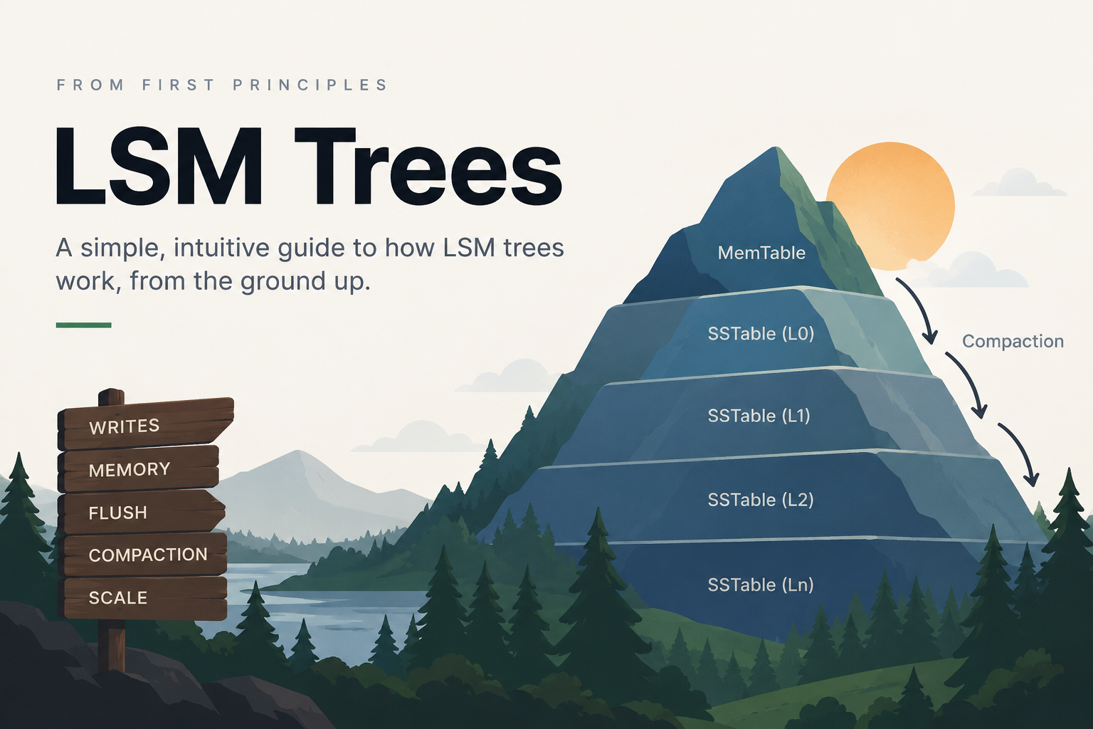
A write follows roughly this path:

User Write
    ↓
  WAL
    ↓
Memtable
    ↓
  Flush
    ↓
SSTable
    ↓
Compaction

Lets Understand All Components in Details

WAL (Write Ahead Logs)

The first problem we need to solve is durability. Our writes are going into the Memtable, which lives in memory. That's fast, but memory is not permanent.

Imagine we receive:

PUT manga:10 Berserk

If we put it directly into the Memtable:

Memtable

manga:10 → Berserk

and the process crashes, the write is gone. So we first record the operation on disk in a Write-Ahead Log (WAL) and then put it into the Memtable:

User Write
    ↓
   WAL
    ↓
Memtable

A WAL is a common durability mechanism used by many databases, including traditional B-Tree-based databases. The idea is simply to record the operation before modifying the actual database state.

The WAL is an append-only log:

PUT manga:10 Berserk
PUT manga:11 One Piece
DELETE manga:12

We don't modify old entries. New operations are appended to the end.

The order is important:

1. Write to WAL
2. Write to Memtable

If the process crashes after step 1, the operation is still in the WAL. When the database starts again, it can replay the WAL and rebuild the Memtable.

WAL
 │
 │ replay
 ▼
Memtable

In my go implementation , we follow the same order.

wal.AddOperation("PUT", key, &value)
memtable.Put(key, value)

Now that the write is safely recorded, we need somewhere to accumulate these writes in memory.

That's the job of the Memtable.

Memtable

Now that the write is safely recorded in the WAL, we need somewhere to keep it while it's still in memory.

That's the job of the Memtable.

A Memtable is an in-memory data structure that holds the latest writes before they are written to disk.

For example:

Memtable

manga:10 → Berserk manga:11 → One Piece manga:12 → Naruto

Because the data is in memory, writes are fast. We don't need to perform a disk write for every operation. The Memtable also keeps its keys sorted:

10 → Berserk 11 → One Piece 12 → Naruto 13 → Monster

This becomes useful when we eventually write the Memtable to disk.

What happens when it fills up? Memory is limited, so the Memtable can't keep growing forever. Once it reaches its size limit, we take its contents and flush them to disk as a new sorted file.

Memtable ↓ Flush ↓ SSTable

The important part is that we don't update an existing file. We create a new SSTable containing the Memtable's data. After the flush, the Memtable can be cleared and start accepting new writes.

Memtable ↓ SSTable 1

Memtable ↓ SSTable 2

Memtable ↓ SSTable 3

This is where the LSM approach starts to become interesting: writes keep creating new immutable files instead of modifying existing files.

So now we have another problem:

What exactly is an SSTable, and how do we store and read these files?

3. SSTable

When the Memtable fills up, we need to move its data to disk.

Instead of modifying an existing file, we write the entire sorted Memtable into a new file.

This file is called an SSTable, or Sorted String Table.

For example, our Memtable might contain:

Memtable

10 → Berserk
11 → One Piece
12 → Naruto
13 → Monster

When it is flushed:

Memtable
    ↓
  Flush
    ↓
SSTable

10 → Berserk
11 → One Piece
12 → Naruto
13 → Monster

The data is already sorted, so we can write it to disk in sorted order.

SSTables are immutable

Once an SSTable is written, we never modify it.

Suppose we later update:

10 → Berserk

to:

10 → Berserk Deluxe Edition

We don't open the old SSTable and change it.

The new value goes through the same process:

WAL
 ↓
Memtable
 ↓
New SSTable

So for some time, we might have:

SSTable 1

10 → Berserk


SSTable 2

10 → Berserk Deluxe Edition

When reading, we check the newest SSTables first. The newer value therefore takes precedence. This is one of the key differences from the B-Tree approach we saw earlier: we don't update old files in place; we keep writing new ones.

But there is a problem

Every Memtable flush creates another SSTable.

After enough writes, we could end up with:

SSTable 1
SSTable 2
SSTable 3
SSTable 4
SSTable 5
...

Now a read may have to check multiple files.

Some of those files may also contain old versions of the same keys.

So we need a way to merge these files and remove data that is no longer needed.

That's where compaction comes in.

4. Compaction

We now have multiple SSTables on disk:

SSTable 1
10 → Berserk
11 → One Piece

SSTable 2
10 → Berserk Deluxe Edition
12 → Naruto

SSTable 3
13 → Monster
14 → Death Note

There are two problems here:

1. A read may need to check multiple SSTables.
2. Older SSTables may contain values that have already been replaced.

We can solve both by merging SSTables together.

This process is called compaction.

SSTable 1 ──┐
SSTable 2 ──┼──→ Compaction → New SSTable
SSTable 3 ──┘

Since each SSTable is already sorted, we can efficiently merge them.

For duplicate keys, the newest value wins:

SSTable 1
10 → Berserk

SSTable 2
10 → Berserk Deluxe Edition

After compaction:

New SSTable

10 → Berserk Deluxe Edition

The older version can now be discarded.

The same applies to deletes. Instead of immediately removing a key from older SSTables, we record a tombstone indicating that the key was deleted. During compaction, that tombstone can be used to remove the older value.

So instead of:

SSTable 1
SSTable 2
SSTable 3
SSTable 4
SSTable 5

we periodically reduce them to fewer, larger files.

SSTable 1 ──┐
SSTable 2 ──┤
SSTable 3 ──┼──→ Compaction
SSTable 4 ──┤
SSTable 5 ──┘
                 ↓
             SSTable 6

The goal is simple:

Keep the number of SSTables manageable and remove old versions of data.

At this point, we have the core LSM Tree write path:

Write
  ↓
 WAL
  ↓
Memtable
  ↓
SSTable
  ↓
Compaction

The next question is now about the read path: if the same key can exist in the Memtable and multiple SSTables, how do we find the correct value efficiently?

Reading and Deleting Data

Now that we have all the components, let's look at what actually happens when we read or delete a key.

Read

A read starts with the newest data and moves towards older SSTables:

GET manga:10
      ↓
  Memtable
      ↓
Newest SSTable
      ↓
Older SSTable
      ↓
    ...

If the key is found, we return the value immediately.

But checking every SSTable can become expensive as the number of files grows.

So we use a Bloom Filter for each SSTable.

Before reading a file, the Bloom Filter tells us whether the key might exist in that file:

GET manga:10
      ↓
  Memtable
      ↓
 Bloom Filter
   /       \
  No       Maybe
  ↓          ↓
Skip      Read SSTable

A No means the key definitely isn't there, so we skip the disk read.

A Maybe means we have to check the SSTable. Bloom Filters can have false positives, but they never have false negatives.

This makes reads much cheaper when we have many SSTables.

Delete

Because SSTables are immutable, we can't simply remove a key from an old SSTable.

Instead, a delete is written as a tombstone:

DELETE manga:10

The tombstone is stored like any other write and eventually ends up in an SSTable.

During a read, if we encounter the tombstone:

GET manga:10
      ↓
SSTable
      ↓
10 → DELETE
      ↓
  Not Found

We stop searching. This prevents an older SSTable from returning a value that has already been deleted.

During compaction, the old value and its tombstone can eventually be removed together.

---

Closing Thoughts

Reading about LSM Trees is one thing, but implementing one makes the trade-offs much easier to understand.

I built a small LSM-based key-value store in Go from scratch to get a better feel for how the pieces actually fit together — from the WAL and Memtable to SSTables, compaction, tombstones, and Bloom Filters.

The implementation is intentionally simple and is meant for learning rather than production use.

You can find the complete project here:

LSM KV Store in Go

The biggest takeaway for me was that an LSM Tree isn't really about one complicated data structure. It's about making a series of trade-offs:

Make writes cheap by avoiding in-place updates, and pay the cost later through compaction.

Once you look at it this way, the different pieces of an LSM Tree start to make a lot more sense.